
A brief explanation of importance sampling
Published:
In this post, I provide a brief overview of importance sampling, a sampling-based method widely used in structural reliability analysis. This classical technique has recently drawn my attention because it is frequently cited in the literature I am currently exploring. Revisiting its underlying concepts offers a valuable opportunity to refresh my understanding of this well-established method, which I was first introduced to during my graduate studies.
Importance Sampling
Structural reliability analysis aims to calculate the failure probability $p_F$ defined by
\[p_F = \int_{\Omega_f} f_{\mathbf{X}}(\mathbf{x}) \, d\mathbf{x}\]where the joint probability density function $f_{\mathbf{X}} (\cdot)$ of the random vector $\mathbf{X}$ is integrated over the failure domain $\Omega_f = \{ \mathbf{x} \mid g(\mathbf{x}) \leq 0 \}$ with $g(\cdot)$ as the limit state function. This can be reformulated as
\[\begin{align} p_F &= \int_{\Omega_f} I( \mathbf{x} ) f_{\mathbf{X}}(\mathbf{x}) \, d\mathbf{x} \\ &= E[I( \mathbf{X} )] \end{align}\]in terms of an indicator function $I( \cdot )$ with $I( \mathbf{x} )=1$ if $\mathbf{x} \in \Omega_f$; otherwise $I( \mathbf{x} )=0$. The failure probability becomes the expectation of the indicator function relative to the distribution of $\mathbf{X}$. Furthermore, this expression can be rewritten in standard normal space
\[\begin{align} p_F &= \int_{\Omega_f} I( \mathbf{u} ) \phi(\mathbf{u}) \, d\mathbf{u} \\ &= E[I( \mathbf{U} )] \end{align}\]where an appropriate transformation $\mathbf{x}= \mathbf{T}^{-1}(\mathbf{u})$ is implemented while $\phi(\cdot)$ is the standard normal probability density function. The importance sampling makes use of the formulation
\[\begin{align} p_F &= \int_{\Omega_f} I[ \mathbf{u} ] \frac{\phi(\mathbf{u})}{h(\mathbf{u})}h(\mathbf{u}) \, d\mathbf{u} \\ &= E_h\left[I( \mathbf{U} ) \frac{\phi(\mathbf{U})}{h(\mathbf{U})} \right] \end{align}\]where $E_h[\cdot]$ gets the expectation from the samples drawn from the distribution of $h(\mathbf{u})$. The main idea of importance sampling is to draw samples from a more important region because sampling away from unimportant regions can be computationally expensive for low failure probabilities. The expression above essentially shifts the sampling distribution from the original sampling distribution $f_{\mathbf{X}}$ or in standard normal space $\phi(\mathbf{U})$ towards the $h(\mathbf{u})$. The next sensible question is how to select the new sampling density $h(\mathbf{\cdot})$. A vast literature provides several options for this sampling-based methodology.
Let $\mathbf{u}_i^{(h)}$ as realizations of samples drawn from the sampling density $h(\cdot)$, an advantage is only gained in using importance sampling when
\[q_i = I\left( \mathbf{u}_i^{(h)} \right) \frac{\phi\left( \mathbf{u}_i^{(h)} \right)}{h \left(\mathbf{u}_i^{(h)} \right) },\:\: i=1,..., n_{samples}\]the variable $q_i$ has a small variance. This is why Importance sampling is referred as a variance reduction technique relative to the crude Monte Carlo simulation approach. Thus, variants of this approach differs with the sampling density. A detailed discussion on selecting sampling density function is provided in Melchers and Beck (2018).
One of the widely implemented approach in importance sampling is provided by Melchers (1989). It is suggested that the sampling density follows a normal distribution centered at the design point (or most probability point) $\mathbf{u}^{*}$ identified by First-Order Reliability Method (FORM) (see Melchers and Beck (2018) for discussion of this method).
\[\mathbf{U}^{(h)} \sim N(\mathbf{u}^{*}, \sigma^2 \mathbf{I})\]with equal variances $\sigma^2=1$. An unbiased estimator of failure probability
\[\begin{align} p_F &\approx \frac{1}{n_{samples}} \sum_{i=1}^{n_{samples}} q_i \\ &= \frac{1}{n_{samples}} \sum_{i=1}^{n_{samples}} I\left[ \mathbf{u}_i^{(h)} \right] \frac{\phi\left( \mathbf{u}_i^{(h)} \right)}{h \left(\mathbf{u}_i^{(h)} \right) } \end{align}\]Algorithm
- Perform FORM and find the design point in standard normal space $\mathbf{u}^{*}$.
- Define number of samples $n_{samples}$
- Draw $\mathbf{u}_i^{(h)}$ samples from $N(\mathbf{u}^{*}, \sigma^2 \mathbf{I})$.
- Transform $\mathbf{x}_i= \mathbf{T}^{-1}(\mathbf{u}_i^{(h)})$ into the real space.
- Evaluate the limit state function at $g(\mathbf{x}_i)$.
- Calculate the value of $q_i$ with $I[\mathbf{x}_i] = 1$ if $g(\mathbf{T}^{-1}(\mathbf{u})) \leq 0$; otherwise $I[\mathbf{x}_i] = 0$. The density functions $\phi\left(\mathbf{u}_i^{(h)} \right)$ is the standard normal PDF and $h\left(\mathbf{u}_i^{(h)} \right)$ is the normal PDF with properties $N(\mathbf{u}^{*}, \sigma^2 \mathbf{I})$.
- Repeat 3-6 for $i=1,..,n_{samples}$.
- The failure probability is calculated as $p_F \approx \frac{1}{n_{samples}} \sum_{i=1}^{n_{samples}} q_i$
Example
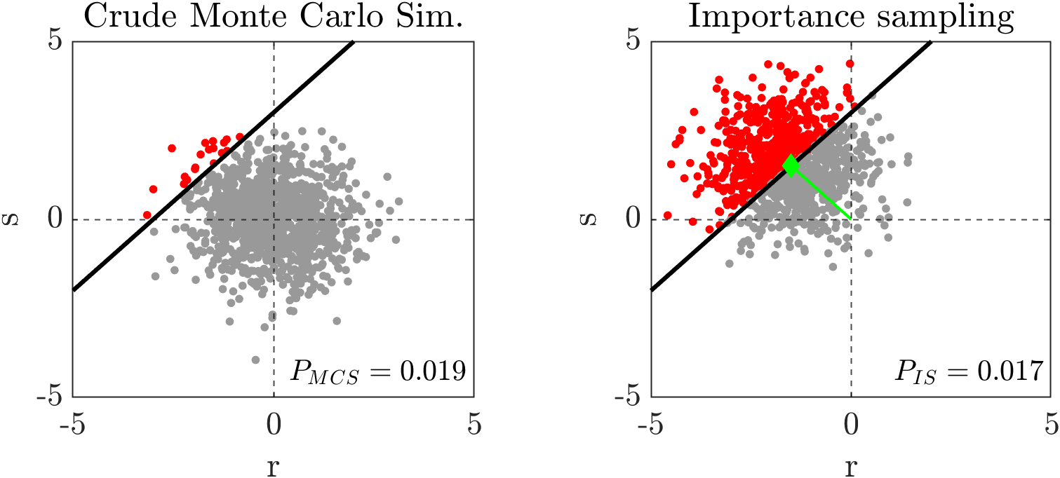
Given random variables $R\sim N(6,1^2)$ and $S\sim N(3,1^2)$. The limit state function is given as $g(R,s)=R-S$. The samples for a Monte Carlo simulation and Importance sampling is shown below. The design point identified $u^* = [-1.5, 1.5]$ or in real space $u^* = [4.5, 4.5]$.
The matlab codes provided here demonstrates on how to perform reliability analysis using Importance sampling.
More discussion about importance sampling is provided in :
Melchers, R. E., & Beck, A. T. (2018). Structural Reliability Analysis and Prediction (2nd ed.). John Wiley & Sons.
Melchers, R. E. (1989). Importance sampling in structural systems. Structural Safety, 6(1), 3–10. https://doi.org/10.1016/0167-4730(89)90003-9{.uri}
Der Kiureghian, A. (2022). Structural and System Reliability (1st ed.). Cambridge University Press. https://doi.org/10.1017/9781108991889